
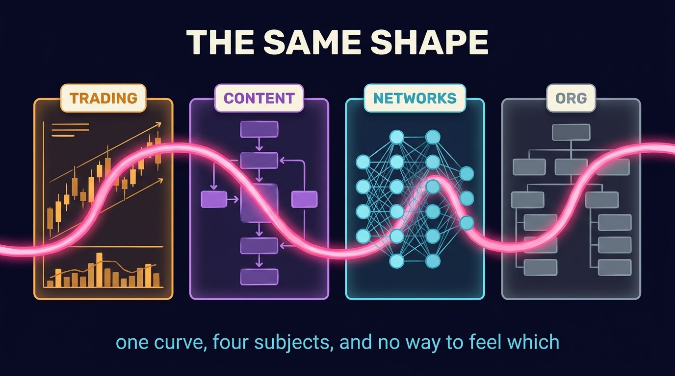
Four systems I built across about ten years had nothing to do with each other. A grid trading strategy running on thin crypto markets. A content production pipeline that turns raw source material into finished long-form work. A knowledge store meant to hold everything I had ever read in a form I could actually query. An operating structure for a portfolio of small companies that all have to run without me watching them.
They kept coming out the same shape. Each one had a point where it had to choose between running the configuration that already worked and spending resources testing one that might work better, and in each one that choice was the hardest part. Each one had a friction term I had originally modelled as a correction, and in each one that term turned out to decide whether the system was viable at all. Each one broke in the same place, at the moment its environment changed faster than its assumptions could be updated, and each one broke worst when the environment was halfway between two states rather than solidly in either.
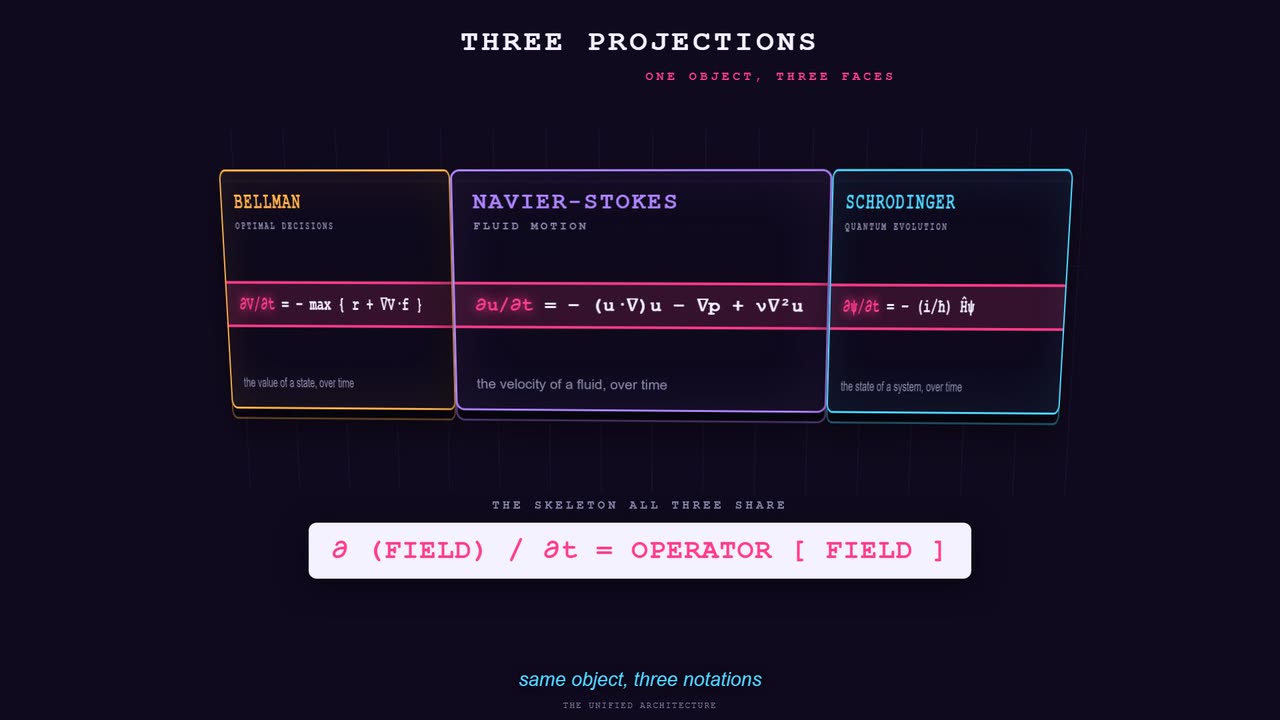
Optimal decision-making, fluid flow and quantum evolution are three projections of one mathematical object, connected by published derivations rather than by resemblance. Once that lands, the tools built for one of them become design primitives for the others, and a decade of noticing the same shape stops being a habit of mind and becomes a thing you can compute with. This entry walks the whole path: the mathematics, the decision layer that falls out of it, the knowledge structure that layer needs, the domain where all three get tested hardest, and the shape everything converges on when you build it for real.
The pattern that kept showing up
Four domains that should not have rhymed
Take the trading case first, because it is the one where being wrong costs money the same week. A grid strategy places a ladder of orders around a price and earns the spread as price oscillates through them. Three parameters decide everything: how wide to space the rungs, how far the ladder extends, and how much capital sits on each rung. Set them for a calm market and a trending one walks straight through the ladder and leaves you holding inventory that keeps falling. Set them for a volatile market and a calm one never reaches your outer rungs, so most of your capital does nothing.
Now the content pipeline, which has no prices in it at all. Raw material comes in unstructured and partly wrong. A sequence of passes narrows it: extraction, structure, drafting, formatting, verification. Every pass depends on the cleanup the previous one did. The interesting parameters are how much context to hand a given pass, how much freedom to give it, and where to put the checks that fail closed. Set those for a source you know well and an unfamiliar one produces confident nonsense. Set them for maximum caution and the output is technically correct and worth nothing.
The knowledge store had the same skeleton wearing a third costume. So did the operating structure, where the parameters are how much autonomy each unit gets and how tight the reporting loop is. In all four, the same question keeps arriving: how much of your resource do you commit to the thing that is currently working, and how much do you spend finding out whether something else works better? In all four, the friction of acting at all (fees and slippage, the cost of a pass, the overhead of a handoff) turned out to be a primary term rather than a rounding error. And in all four, the dangerous moment was never the calm regime or the wild one. It was the boundary, where a system tuned for one was still running while the other arrived.
The problem with noticing things
Here is the difficulty with that observation, and it is the reason this entry exists rather than a shorter one. Seeing structure across unrelated domains is exactly what a mind does when it is working well and exactly what it does when it is malfunctioning. The clinical word for the malfunction is apophenia: perceiving meaningful connections between unrelated things. From inside, a real cross-domain pattern and a false one feel the same. Both arrive as recognition. Both come with the pleasant certainty that you have understood something other people have missed, and that certainty is worth nothing as evidence, because it is produced by the same machinery in both cases.
I have the kind of brain that does this constantly. Some of it is useful and some of it is noise, and for most of that decade I had no reliable way to sort one from the other. Every framework I found made the sorting harder rather than easier, because a good framework can be applied to anything, and a thing you can apply to anything tells you nothing about what you applied it to. Petri nets, promise theory, Wardley maps, game theory: each one looked like the master key for about a month.
What settles the question is external and specific. Either there is a derivation connecting the two domains, written down by someone who was not trying to make a point about my portfolio, checkable by anyone who knows the mathematics, or there is not. If there is, the shared structure is a fact about the equations and the resemblance you noticed was a shadow of it. If there is not, you have a metaphor, which is a fine thing to have as long as you never build on it.
What this entry covers, and how it is grounded
The derivation exists. It runs from the Bellman equation through its continuous-time form to the equations of fluid motion, and out sideways into quantum mechanics, and every step of it is published work by mathematicians with no interest in trading systems or content pipelines. The next four sections walk that chain slowly, in plain language first and notation second, and mark clearly where a result is settled consensus and where it is one author's specific formulation.
After that the entry moves outward in one direction: from the mathematics to a decision layer that partitions every policy in any domain into exactly four classes, to the knowledge structure that layer needs in order to reason about its own reasoning, to quantitative finance as the proving ground where the whole stack gets tested against an adversary that does not care about your framework, to the shape all of it converges on when built, which turns out to be a compiler, and finally to what that shape does to the economics of a small operation.
One commitment about method, made here because the rest of the entry leans on it. Every number below is either linked to a source, or shown as arithmetic with its assumptions on the page, or marked as my own judgment. An argument that rests on published derivations has no business smuggling in figures that rest on nothing, and the claims in this entry that are mine rather than the literature's are labelled as mine.
Bellman, and the crossroads
Imagine you are standing at a crossroads. Each path leads to a different destination, and each destination has its own crossroads with its own paths. You do not know exactly what lies ahead, and you do know that every choice you make now shapes which choices become available later. The question is how you pick the best path when the map is too large to see all at once.
The equation that answers it
This is the problem Richard Bellman formalised in the 1950s. What he wrote down is simple enough to feel like a tautology on first read, which is part of why it took so long for anyone to write it down:
V(s)  =  maxa  E[ reward(s, a)  +  γ · V(s') ]

V(s)          the value of being in state s
max over a    across every action available to you here
E[ ]          in expectation, because the outcome is uncertain
reward(s,a)   what that action pays you immediately
γ             the discount factor, between 0 and 1
V(s')         the value of the state that action leaves you in
In plain language: evaluate each path by adding what you get right now to the best thing you can get from wherever that path leads. Pick the path with the highest total. Then do that recursively at every crossroads, and you have an optimal strategy for the entire network rather than a good move at one junction.
The recursion is the part that earns its keep. The value of a state is defined in terms of the values of the states it leads to, which means a decision made now carries the consequences of every decision it makes available later, without anyone having to enumerate those consequences by hand. A grid trader widening the spread on a thin token is solving this whether or not the word Bellman ever enters their head: the immediate reward is fee capture on the trade, and the discounted future value is the position that trade leaves them holding, with its inventory risk and its opportunity cost.
The discount factor is doing real work
That gamma is easy to read as a modelling convenience. It is a claim about the world. A reward three steps out is worth less than the same reward now, because the intervening steps can fail, the environment can move, and the counterparty can disappear. The discount factor is where a system encodes how much it believes its own forecasts.
Set gamma near zero and you have built something that grabs whatever is in front of it and never invests. Set it near one and you have built something that will accept unbounded present cost for a future it has no ability to guarantee. Neither extreme is a tuning error so much as a statement about the environment, and the same knob appears in every domain in this entry: how far ahead a content pipeline optimises before it ships, how long a company waits for a capability to pay off, how many rungs out a ladder of orders extends before the outer rungs stop being worth the capital parked on them.
The curse Bellman named himself
Bellman also identified the obstacle that stops you computing this exactly, and he named it with some flair: the curse of dimensionality. As the number of variables describing your state grows, the number of possible states grows exponentially rather than proportionally.
The arithmetic is worth doing once, because the scale of it explains an entire industry's design choices. Take a trading system watching 50 tokens, tracking 4 quantities on each one (price, volume, a regime indicator, a liquidity measure), and discretising each quantity into 20 buckets. Those are my assumptions, chosen to be modest rather than adversarial:
50 tokens × 4 quantities            =  200 state dimensions
20 buckets per dimension          =  20200 distinct states

20200  =  10(200 × log₁₀ 20)  =  10(200 × 1.301)  ≈  10260

for scale: the observable universe holds roughly 1080 atoms
A table with one row per state is impossible by a margin of 180 orders of magnitude. Which is why every reinforcement learning system you have heard of approximates the value function instead of computing it: neural networks, gradient-boosted trees, linear function approximators. The approximation is forced by the size of the space rather than chosen for convenience, and every argument later in this entry about which policy class to use is downstream of that forcing. The decision-theory entry on intelligence engineering takes the approximation question further into search and tree methods; here the point is only that exactness left the building early and nothing since has invited it back.
Shrink the step and the equation changes character
The Bellman equation works in discrete steps. Turn left or right. Buy or sell. Run the pass or hold. Real environments rarely have the courtesy to be discrete. Price evolves continuously, liquidity shifts between your ticks, and an agent that only thinks when a candle closes is asleep for the interval between closes.
So shrink the timestep toward zero and apply a Taylor expansion. What comes out is the Hamilton-Jacobi-Bellman equation, a nonlinear partial differential equation giving necessary and sufficient conditions for optimal control in continuous time. The question it answers has changed shape. Bellman asks what the best move is at this step. HJB asks what the best trajectory is through a landscape that is deforming while you cross it.
| RESOLUTION | WHAT IT OPTIMISES | WHAT IT CANNOT SEE |
|---|---|---|
| Bellman, discrete | the best action at each decision point | everything happening between decision points |
| HJB, continuous | the best trajectory through a moving landscape | nothing structurally, at the cost of solving a nonlinear PDE |
The gap between those two rows is operational rather than academic. A system working at discrete resolution is blind between its ticks, and microstructure signals that live inside the interval are unavailable to it at any price. Raising the tick rate narrows the blindness without removing it. Moving to the continuous formulation removes the interval entirely, which is the whole reason the next four sections are about a partial differential equation rather than a lookup table.
One more property of HJB matters for everything downstream. It is stated on a space of trajectories rather than a list of states, which means the objects it operates on can be strange: paths through a configuration space, rearrangements of a medium, allocations of a fixed budget across a network. That generality is what lets the next section pick up a completely different subject, fluid motion, and arrive back at the same equation from the other side.
Water in a pipe
Set decision-making aside completely for a moment and think about water moving through a pipe. Nothing in this section is about markets or agents. The connection arrives in the section after it, and it arrives as a derivation rather than a comparison, which only works if the fluid mechanics is understood on its own terms first.
Four forces on every parcel
The Navier-Stokes equations describe how fluids move. Every river current, every weather system, every aerodynamic simulation, every swirl of milk entering coffee is governed by them. What they express is a force balance applied to every infinitesimal parcel of the fluid, continuously, everywhere at once.
ρ(∂u/∂t + u·∇u)  =  −∇p  +  μ∇²u  +  f

ρ(∂u/∂t + u·∇u)   inertia. the parcel's tendency to keep doing what it is doing
−∇p                pressure. high pushes toward low, everywhere, always
μ∇²u               viscosity. internal friction, dragging neighbours toward agreement
f                   external forcing. gravity, a pump, wind across a surface
Read the left side as what the parcel wants to do and the right side as everything acting on it. The term that makes the whole system difficult is the second half of the inertia group, u·∇u, where the velocity field acts on itself. Fast-moving fluid creates pressure gradients that create more movement that creates more gradients. That self-reference is the source of everything interesting in fluid dynamics and the reason the mathematics resists solution: turbulence, eddies, weather, and a two-century-old open problem all come out of one nonlinear term.
Nearly two centuries old, and still open
The equations date to the 1820s to 1840s, and nobody has proved whether smooth, physically sensible solutions always exist in three dimensions. The Clay Mathematics Institute lists existence and smoothness for Navier-Stokes as one of its seven million-dollar Millennium Problems, and as of 2026 the prize remains unclaimed, with neither a proof of global regularity nor a construction of finite-time blowup accepted.
The practical status is worth stating alongside the theoretical one, because they diverge and the divergence is instructive. Engineers solve these equations numerically every day to design aircraft wings, forecast weather and model blood flow, and the answers are good enough to bet lives on. What is unresolved is whether the equations can ever produce something physically impossible, such as velocity concentrating to infinity at a point in finite time. A discipline can be enormously productive while its foundations remain open, which is a pattern that recurs in every field this entry touches.
Viscosity carries the same standing as inertia
One detail governs everything downstream. Viscosity sits in the equations as a primary force term, with the same standing as inertia and pressure. You cannot compute a real flow without modelling internal friction, because frictionless fluids do not exist in reality. Superfluid helium near absolute zero is the exception that proves how exotic the conditions have to be.
Drop the viscous term and the equations do not become an approximation of a real fluid. They become the Euler equations, which describe a different, idealised object that behaves qualitatively differently: no boundary layers, no drag on a body moving through it, no dissipation of energy at small scales. Aerodynamics spent decades on this exact confusion, because the idealised theory predicted that a wing generates no drag, which is an interesting result about the model rather than about wings.
| FLUID TERM | WHAT IT IS IN A MARKET | WHAT IGNORING IT COSTS |
|---|---|---|
| Inertia | momentum, trend persistence, flow that keeps going because it is already going | you treat every move as noise around a mean that is quietly relocating |
| Pressure | order book imbalance, the gradient between resting bids and asks | you model price without modelling what is pushing it |
| Viscosity | fees, spread, slippage, market impact. every cost of acting | a strategy that is profitable on paper and negative in production |
| External forcing | news, unlocks, listings, liquidations, anything arriving from outside | you attribute an exogenous shock to a flaw in your own model |
Transaction costs are the viscosity of a market, and viscosity is a primary term. A model that subtracts fees at the end from a strategy designed without them has computed the optimal path for a frictionless medium and then charged it rent. The section on the seven sins comes back to this with the specific failure it produces; the point to carry from here is structural. Friction belongs in the equation you optimise, at the point where you optimise it.
The one number that tells you which world you are in
Given four competing forces, the useful question is which one dominates, and fluid dynamics answers it with a single dimensionless ratio. The Reynolds number is inertial forces divided by viscous forces, and it is the most consequential quantity in the field.
Re  =  ρuL / μ   =   inertial forces / viscous forces

Re < ~2,000      laminar      smooth parallel layers. honey from a jar.
~2,000 - 4,000   transitional  unstable, flickering between the two
Re > ~4,000      turbulent     chaotic eddies at every scale. white water.
Low Reynolds means friction wins and the flow moves in smooth parallel layers, predictable and exploitable. High Reynolds means momentum wins and the flow breaks into eddies and vortices, rich with structure at every scale, statistically characterisable, and impossible to predict in detail. Between the two thresholds the flow is genuinely unstable, flickering between states, and the thresholds themselves are conventions from pipe-flow experiments rather than universal constants.
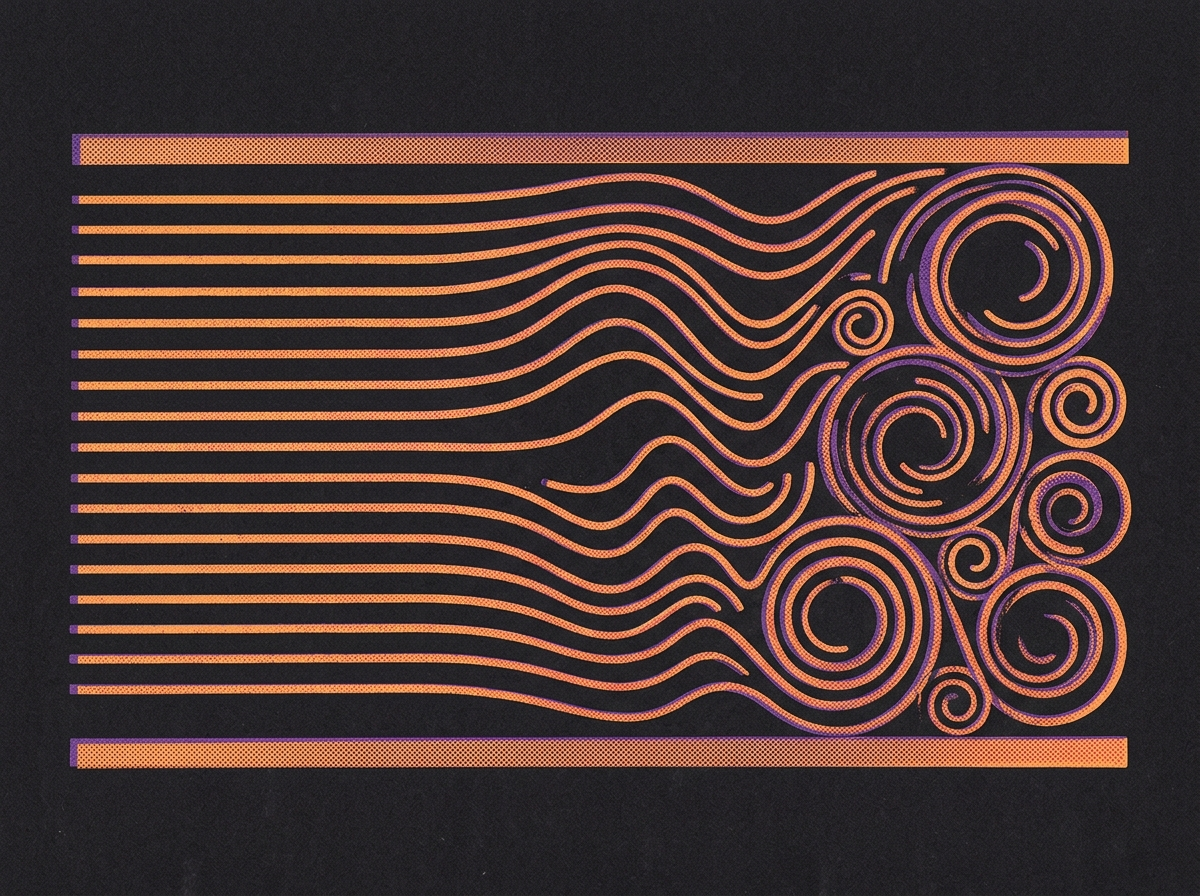
Hold that middle band in mind. It is the most dangerous region in fluid dynamics and, once the connection in the next section is established, the most dangerous region for any system that has been tuned to a regime.
Turbulent does not mean random
One correction to make now, because two later sections depend on it and the everyday use of the word points the wrong way. Turbulence is not noise. It is highly structured motion whose structure lives at many scales simultaneously, and the structure is stable enough to have quantitative laws written about it.
Kolmogorov's 1941 description is the standard picture. Energy enters a flow at a large scale, at the size of the pipe or the wing or the storm. It does not dissipate there, because viscosity is far too weak at that scale to absorb it. Instead the large eddies break into smaller eddies, which break into smaller ones again, passing energy down through the scales in a cascade. Viscosity only becomes strong enough to convert motion into heat at the very bottom, at a size called the Kolmogorov microscale, which is set by how much energy is arriving and how viscous the medium is. Between the top and the bottom sits an inertial range where the statistics follow a power law that does not care about either end.
Two consequences carry forward. A cascade means the same kind of structure repeats across scales rather than each scale doing its own unrelated thing, which is why a measurement taken at one resolution says something about a different resolution. And the microscale is a real floor: below it, friction dominates absolutely and organised motion cannot persist. Both of those come back later, the first when the econophysics literature finds cascade structure in exchange rates, the second when the same arithmetic sets a minimum spacing below which a trading grid cannot profit no matter how it is tuned.
So the laminar and turbulent labels sort flows by which kind of predictability is available, rather than sorting them into predictable and unpredictable. A laminar flow is predictable in detail: you can say where this parcel goes. A turbulent flow is predictable in distribution: you can say how energy is spread across scales and how often a fluctuation of a given size occurs, while saying nothing about any individual eddy. Those are two different products and they demand two different kinds of system to exploit them, which is the substance of the exploration and exploitation argument several sections from here.
The theorem, and where analogy stops
Here is where the ground shifts. Two subjects have been developed separately: optimal sequential decision-making, which produced the Bellman equation and then HJB, and fluid motion, which produced Navier-Stokes. They were built by different people for different reasons in different centuries. The claim of this section is that they are the same equation viewed from two positions, and the claim is carried by derivations rather than by the resemblance that made anyone look.
Arnold, 1966: a fluid takes the shortest path
Start with the fluid side. In 1966 Vladimir Arnold published a geometric reformulation of ideal incompressible flow. The set of all the ways an incompressible fluid can rearrange itself while conserving volume is a mathematical object in its own right: an infinite-dimensional group, written SDiff(M), whose elements are volume-preserving diffeomorphisms of the region M the fluid occupies. Give that group a metric built from kinetic energy, and Arnold's result says that the motion of an ideal fluid traces a geodesic, the shortest available path, through that space. Ebin and Marsden made the argument rigorous in 1970 using infinite-dimensional Riemannian geometry.
Take a moment with what that means physically, because it is easy to read past. A fluid does not deliberate. Nothing in a river is choosing. And the trajectory a river takes through the space of all possible rearrangements of itself is the one that minimises a cost, in exactly the sense a shortest path minimises distance. The optimisation language describes the physics rather than decorating it, and that description turned out to be equivalent to the original one. It opened a large research literature on Euler-Arnold equations, since many other nonlinear evolution equations in mathematical physics fit the same template.
Arnold's theorem covers the ideal case, meaning no viscosity. That restriction matters, given how much weight the previous section put on viscosity being a primary term, and it is exactly where the next result comes in.
The step that closes the loop
Now bring the decision side to the same space. Xiang-Dong Li and Guoping Liu's paper On the Navier-Stokes equations and the Hamilton-Jacobi-Bellman equation on the group of volume preserving diffeomorphisms, published in SIAM Journal on Control and Optimization, does precisely this. Their abstract states the result plainly: they give "a new derivation of the incompressible Navier-Stokes equations on a compact Riemannian manifold M via the Bellman dynamic programming principle on the infinite dimensional group SG = SDiff(M) of volume preserving diffeomorphisms," and note that "when the viscosity vanishes, we give a new derivation of the incompressible Euler equation."
That is the whole load-bearing claim of this entry, stated by mathematicians in a control-theory journal. Apply the optimal-control machinery to the space of volume-preserving rearrangements and the incompressible Navier-Stokes equations come out, viscosity included. Set viscosity to zero and you recover Arnold's geodesic picture as the special case. Their paper also relates both to the viscous Burgers equation on the same group, which is the technical bridge that makes the derivation work.
This sits inside a longer line of work rather than arriving alone, which is the sort of thing that raises confidence rather than lowering it. Cipriano and Cruzeiro gave a stochastic variational principle for two-dimensional incompressible Navier-Stokes using Brownian motion on a group of homeomorphisms; Arnaudon and Cruzeiro extended it to general compact Riemannian manifolds; Constantin and Iyer built a stochastic Lagrangian representation on the same objects. Several independent routes arrive at the same place: solutions of Navier-Stokes are critical points of a control problem posed on the group of volume-preserving maps.
What this licenses, and what it does not
Precision here protects everything downstream, so two separations are worth making explicitly.
What is established: the mathematical identity above. Optimal control on SDiff(M) yields incompressible Navier-Stokes; the ideal case recovers Arnold. That is published, refereed, and checkable by anyone with the background, and it holds regardless of what anyone builds with it.
What is a specific author's programme rather than settled consensus: the claim that this identity should be used as an engineering substrate, that attention or computational budget flowing through a network is usefully modelled as an incompressible fluid, and that the resulting architecture behaves the way its designer expects. That is Ben Goertzel's FluQNet framework, and it is a research proposal with a mathematical foundation rather than a deployed and validated technology. Both facts are load-bearing in this entry, and conflating them would be the exact error the first section spent 1,200 words describing.
What the identity does license is concrete and worth naming. If routing a fixed budget through a network is an optimal-control problem on volume-preserving maps, then Reynolds numbers, viscosity, boundary layers, laminar and turbulent regimes and cascade scaling become available as design primitives for decision systems, carrying their existing quantitative content with them. You are borrowing a century of applied mathematics with the derivation attached rather than borrowing vocabulary.
Complexify, and a third face appears
The triangle closes with quantum mechanics, and the mechanism is older and more mundane than the destination suggests.
Take the HJB equation and apply a logarithmic transformation to the value function. For a specific class of control problems, where a matching condition between the control cost and the noise holds, that transformation linearises the equation. This is the Cole-Hopf transform, and the linear object it produces is a diffusion equation, which is the Schrodinger equation in imaginary time. A Wick rotation, the formal substitution that swaps imaginary time for real time, carries it the rest of the way. The historical detail is that Schrodinger himself used this logarithmic transformation to relate the Hamilton-Jacobi theory to his own equation, so the connection is not a modern reinterpretation so much as a return to the route the equation originally came in by.
The qualifier belongs in the same breath as the result. The linearisation holds for the linearly-solvable class of control problems, rather than for every HJB equation, which is why path-integral control methods work beautifully where the matching condition applies and do not exist elsewhere. Anyone told that decision theory simply is quantum mechanics has been sold a stronger claim than the mathematics supports.
There is an independent route to the same place from 1966, which is the same year as Arnold's paper. Edward Nelson's stochastic mechanics starts from classical Newtonian mechanics, adds a Brownian diffusion with constant proportional to Planck's constant over mass, and derives the Schrodinger equation without presupposing quantum theory. A quantum particle's motion becomes a classical velocity plus a fluctuating component, and quantum behaviour is what classical mechanics looks like once noise of that specific magnitude is present.
Nelson's programme has a known unresolved objection, and stating it is more useful than omitting it. Wallstrom showed that stochastic mechanics recovers the Schrodinger equation only if an additional quantisation condition is imposed on the solutions, a condition that does not fall out of the stochastic framework itself. Work continues on whether that condition can be motivated rather than assumed. So the derivation is real and the equivalence is incomplete, which is a considerably more interesting position than either "quantum mechanics is just noisy classical mechanics" or "the connection is numerology".
The completed picture, at its actual strength. Optimal decisions, fluid motion and quantum evolution are three notations over one mathematical structure, joined by transformations that are written down and checkable. The decision-to-fluid link is a theorem on a specific group of maps. The decision-to-quantum link is a transformation valid on a specific solvable class, with an independent 1966 route that carries an open objection. Reinforcement learning, fluid dynamics and quantum mechanics are three languages for the same mathematics, and knowing which sentences translate cleanly is the difference between using that and merely enjoying it.
The Reynolds number as a dial you can compute
The previous section established an identity. This one spends it, on the oldest open problem in reinforcement learning.
A tradeoff with one clean case and heuristics everywhere else
Every agent that learns faces the same question at every step: run the strategy that is currently paying, or spend this step finding out whether something else pays better. Commit fully to exploitation and you lock in whatever local optimum you stumbled into first. Commit fully to exploration and you never collect on anything you learn.
There is exactly one clean answer in the literature, and its cleanliness comes from its assumptions. The Gittins index theorem solves the classic multi-armed bandit optimally: with independent arms, a fixed discount factor and stationary reward distributions, you can compute an index for each arm separately and simply play the highest. That result decomposed a problem everyone believed was intractable, and it holds only inside those assumptions. Let the arms correlate, let the payoffs shift over time, let context enter, and index optimality departs. What remains is a large family of heuristics (epsilon-greedy, upper confidence bounds, Thompson sampling, entropy bonuses) that are each defensible, each tunable, and none universal.
So practitioners tune. A parameter gets set to a value that worked in testing, and it stays there while the environment underneath it moves. The tuning problem is that the correct amount of exploration is a property of the environment rather than a property of the algorithm, and nothing in the standard toolkit measures that property directly.
The dial, and what goes into it
Fluid dynamics has measured exactly that property for a century, because the Reynolds number is the ratio of the tendency to keep moving to the friction resisting movement. Goertzel's framework takes the identity from the last section and reads the ratio as a control parameter: in his phrasing, a Reynolds-like or Peclet-like number acts as an explicit explore and exploit dial.
Re  =  velocity / viscosity   (schematically, with the scale term folded in)

velocity    how fast the decision environment is changing
viscosity   how much friction resists acting on that change

both sides are observable quantities in a running system, which is
the entire point. neither is a hyperparameter you choose.
The character of the quantity changes when you compute it rather than choose it. An exploration rate set by hand is a claim about the environment made by a person who last looked at it during testing. A ratio computed from live measurements is a claim about the environment made by the environment. The tradeoff stops being a hyperparameter and becomes a reading, which is the difference between a thermostat and a person deciding each morning how warm the house should be based on how warm it was last month.
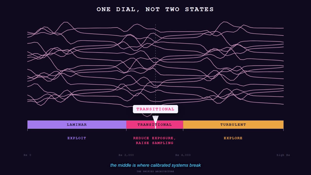
The mapping, regime by regime
| FLOW REGIME | DECISION POSTURE | WHAT IT LOOKS LIKE IN A RUNNING SYSTEM |
|---|---|---|
| Laminar, viscosity dominates | exploit | established parameters run untouched. spreads are predictable, the pass configuration that worked yesterday works today, and probing costs more than it returns. |
| Transitional, neither dominates | reduce exposure, raise sampling | the structure the system is tuned for is dissolving while it is still being traded on. the most expensive place to hold a confident position. |
| Turbulent, inertia dominates | explore | structure exists at every scale and none of it is the structure from last week. probing pays, because the information gradient is steep and stale parameters are worthless. |
Read the middle row twice. It is the one that costs money, and it is the one a two-state classifier cannot represent at all, since a system that recognises calm and wild has to call the boundary one or the other and will be wrong for the whole duration of the crossing.
Why the middle band eats systems
Think about what a regime classifier actually is. It is a model fitted to historical data, which means fitted to regimes that have already finished. It performs well when the current regime resembles a past one, which is most of the time, and it produces exactly the wrong answer during a transition, which is the small fraction of the time when the answer matters most. The failure is not an accuracy problem to be improved with a better model class. It is structural: the classifier's evidence is drawn from a distribution the market has left.
This is the single most useful thing the fluid framing buys, so it is worth stating on its own. A regime is a continuous position on a spectrum rather than a label to be assigned, and the dangerous band has its own name and its own posture. A system that computes where it sits can act differently while it is crossing, instead of holding a confident classification right up to the moment the classification stops being true.
The same reading applies well outside markets. A content pipeline whose source material has started arriving in a new shape is in a transitional regime, and its correct response is to widen its checks and reduce how much it produces per pass. A team whose environment has begun moving faster than its planning cycle is in a transitional regime. In both cases the instinct is to keep running the configuration that has been working, and in both cases that instinct is the failure.
What makes any of this actionable is that the ratio is computable from quantities a running system already observes. The specific market form, price velocity and volume over effective transaction cost, arrives later in this entry alongside the failure it is designed to dissolve. The general form is the one to carry forward: measure how fast your environment moves, measure what it costs you to act, and let the ratio between them set your posture rather than setting it yourself in advance.
One problem, many names
The mathematics of the previous sections describes what an optimal decision is. It says nothing about how to compute one, and the gap between those is where every real system lives. Warren Powell spent a career at Princeton building the bridge, and the first half of his work was diagnosis rather than construction.
A Balkanised field
What he watched was several research communities studying the same problem while remaining largely invisible to each other, because each had built its own notation, its own journals and its own idea of what the problem was called. His own description of the landscape is blunt: the field became "fragmented into a Balkanized set of communities with competing algorithmic strategies and modeling styles", where researchers spend careers inside a single perspective "without recognizing the common themes."
| COMMUNITY | WHAT IT CALLS THE PROBLEM |
|---|---|
| Operations research | stochastic optimization, stochastic programming |
| Computer science | reinforcement learning |
| Control engineering | optimal control, model predictive control |
| Economics | dynamic programming |
| Statistics | bandit problems, sequential design of experiments |
| Simulation | simulation optimization, ranking and selection |
Powell reaches for the parable of the blind men and the elephant. One community grabs the trunk and reports a snake. Another grabs a leg and reports a tree. A third finds the tail and reports a rope. Every report is accurate about the part in hand and useless about the animal. The elephant is sequential decision-making under uncertainty: you observe a state, you decide, information you did not control arrives, the state changes, you decide again. That structure covers a fleet routing trucks through uncertain traffic, a person navigating an unfamiliar business culture, and an algorithm adjusting a ladder of orders while the market moves underneath it.
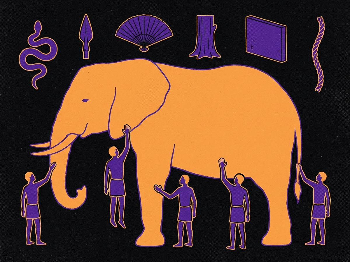
His Reinforcement Learning and Stochastic Optimization (Wiley, 2022) runs to 1,136 pages and adds no new technique. It reorganises the accumulated pile into one structure, proposing "sequential decision analytics" as the name for the unified field, and his framing of the contribution is generous about where the material came from: standing on the shoulders of giants, bringing prior approaches together and looking for cross-pollination that the notation had been hiding.
Five components, one canonical model
The unification runs through a canonical model with exactly five parts. Any sequential decision problem, in any field, gets written down this way.
1  state variables        everything you know at the moment of deciding
2  decision variables     the action you are choosing among
3  exogenous information  what arrives afterward that you do not control
4  transition function    how the state becomes the next state
5  objective function     what you are maximising across the horizon
The move that makes the framework general is in what gets optimised. You do not optimise over decisions. You optimise over policies, meaning functions that map states to decisions. The unit of analysis becomes the rule rather than the choice, which is what connects this layer to the Bellman equation: Bellman gives you a way to evaluate a policy, and Powell gives you a complete account of what kinds of policy there are.
The two questions that partition everything
Ask two binary questions about any policy. Does it use only information available right now, or does it look ahead into the future? Does it compute a direct mapping from state to action, or does it solve an optimisation problem at decision time? Two questions, two answers each, four cells.
                    direct mapping        solves an optimisation

current info only   PFA                   CFA
looks ahead        VFA                   DLA
The four classes, and what each one costs
| CLASS | WHAT HAPPENS AT DECISION TIME | ALGORITHMS THAT LIVE HERE |
|---|---|---|
| PFA policy function approximation | evaluate a tuned function and act. no optimisation, no lookahead, no value estimate. cheapest and most transparent. | lookup tables, rule trees, policy gradient methods such as REINFORCE, any neural net mapping features straight to an action |
| CFA cost function approximation | solve a small parameterised optimisation using only current information. the dials are tuned offline, the choice is made now. | greedy methods with calibrated heuristics, myopic optimisation, index policies such as Gittins |
| VFA value function approximation | estimate the downstream value of the state each action leads to, then act on the estimate. this is where the Bellman equation lives. | Q-learning, deep Q-networks, temporal difference learning, the critic half of actor-critic |
| DLA direct lookahead | build a model of the future, simulate trajectories through it, take the first action of the best plan, discard the rest, repeat. most expensive by a wide margin. | Monte Carlo tree search, rolling horizon optimisation, model predictive control |
Powell's own claim for the partition is that it is universal, in the sense that any method for making decisions belongs to one of the four classes or to a hybrid of them. That last clause carries weight and gets dropped in most retellings. Actor-critic is a PFA whose parameters are trained against a VFA. PPO is a policy search over PFAs using value estimates for advantage. Hybrids are compositions of the four rather than exceptions to them, which is what keeps the partition meaningful while covering methods that visibly do two things at once.
The community that grabbed the trunk
Powell is pointed about one consequence, and it is the practically useful part of his critique. The reinforcement learning community concentrated overwhelmingly on VFA and came to treat that class as the whole subject, which is the blind men problem recurring inside the field that was supposed to have solved it.
Against that, his own record from decades of industrial work in logistics, trucking and energy is that well-tuned PFAs and CFAs frequently outperform sophisticated approximate dynamic programming on real problems. The reason is the one that runs through this entire entry. A simple policy has few parameters and therefore few ways to be wrong about a distribution that has shifted, while a value function approximated over a high-dimensional space inherits several curses of dimensionality at once and degrades when the world stops matching the data it was fitted to.
Carry one operating rule out of this section. Reach for the cheapest class that clears the bar, and climb only when the environment makes the cheaper class fail. Sophistication is a cost paid in fragility as well as in compute, and the class you need is set by how fast your environment moves, which is the ratio the previous section made computable.
The same four classes in five places
Four classes defined by two binary questions is a clean piece of taxonomy and, stated that way, easy to file and forget. What makes it worth building on is that the classes describe a progression people actually climb, in order, whenever they get good at something unfamiliar.
One person, four levels, one city
Take cross-cultural business navigation, which has no equations in it anywhere. Someone lands in Tokyo for a first round of meetings and comes back repeatedly across a few years.
PFA, the tourist. Someone bows, you bow back. A card arrives with two hands, you receive it with two hands. Shoes come off at the door, so yours do too. Observe pattern, replicate pattern. There is no reasoning about why the bow happens, what its depth communicates, or what getting it wrong would cost. The brain computes a direct mapping from an observed state to an action and executes it. The cost is minimal and the result is adequate, which is exactly the profile of a policy function approximation.
CFA, the calibrator. Stay longer and the variation becomes visible. Bow depth moves with relative status, age and the formality of the setting. Gift exchange has parameters: the value, the wrapping, the timing, the number of polite refusals before acceptance. The action space has revealed itself to be continuous rather than discrete, so the person starts tuning dials instead of matching patterns. This is the distance between a phrase book and a conversation.
VFA, the strategist. The qualitative shift happens here, when the question changes from what people do to why the norm exists and what it produces over time. A four-hour dinner where no business is discussed stops looking like a long evening with no return and starts looking like what it is: the host demonstrating commitment through the venue, the attention to preferences, the sheer allocation of time, and the whole thing functioning as an investment in trust that makes every later negotiation cheaper. The person operating at this level is weighing an immediate cost against a discounted future value, which is the Bellman equation running on a human substrate.
DLA, the simulator. The most expensive level runs someone else's decision process inside your own head. Given what you know about a specific counterpart's values, the cultural parameters he operates under and the rules he follows, what does he do if you take a particular action? Choosing to mention the quality of his venue when you meet his superior next week, because you have modelled what that does for his internal narrative, is a direct lookahead: simulate the trajectories, act on the best one, discard the plan when new information lands.
Why most people stop at the first level
Most people never leave PFA in most domains, and the reason is economic rather than a failure of curiosity. The brain defaults to the cheapest strategy that achieves an acceptable result, and climbing a class costs real resources that only pay back when the engagement deepens enough to need them.
That economy also sets the ceiling in the other direction. Powell's own point about the most expensive class is that a theoretically optimal computation taking ten minutes is worthless when the situation changes every five. The right class is set by the environment rather than by how sophisticated you are capable of being, which is the same conclusion the Reynolds section reached from the physics side and is why these two chapters belong next to each other.
| DOMAIN | PFA | CFA | VFA | DLA |
|---|---|---|---|---|
| Cross-cultural navigation | bow when they bow. shoes off at the door. replicate what you observe. | calibrate bow depth by relative status. tune gift value by closeness. | read the four-hour dinner as a trust investment that compounds for years. | simulate the counterpart's decision process before acting. |
| Grid trading | drawdown past the threshold flattens the book. circuit breakers fire without analysis. | optimise spacing, range and allocation for the regime in front of you. | weigh a short-term drawdown against the long-run value of staying deployed. | simulate many stochastic price paths and compute ruin probability before a config goes live. |
| Content production | follow the style guide. apply the template. zero em dashes. run the checklist. | tune depth and framing for this cluster. calibrate length to the actual search intent. | invest in work that ranks in six months, and build authority that compounds. | model topic clusters and gaps across the competitive landscape before commissioning. |
| Agent workflows | a hook blocks a forbidden edit. project rules fire unconditionally. | tune agent parameters per task type. calibrate tool permissions by role. | pay the cost of recording decisions now because it pays back across hundreds of later sessions. | simulate which capability to build first and what the portfolio looks like a year out. |
| Portfolio strategy | non-negotiable conventions. lint gates. pipeline integrity checks. | tune per-company parameters: positioning, pricing, tool selection. | which rung of the ladder each unit is on, and when it climbs. | simulate the portfolio's evolution under resource constraints and market uncertainty. |
Why the mapping is structural
The reasonable first reaction to a framework spanning five domains is suspicion, and the suspicion has a specific shape: you are using a trading vocabulary as a metaphor for cultural navigation, which is a party trick rather than a finding. Taking that objection seriously is the point of this section.
The answer is that the partition is defined by the mathematical structure of the decision, with no reference to the domain anywhere in the definition. Does the policy use only current information, or look ahead? Does it map directly, or optimise? A tourist bowing back is executing a policy function approximation in the full technical sense, since the brain is computing a direct state-to-action mapping with no optimisation, no value estimate and no simulation. The fact that Powell developed the taxonomy against freight logistics gives trucks no better claim to it than the dinner has. The mathematics has no way of telling them apart, because the only inputs to the classification are the two questions.
This is the same species of claim as the theorem several sections back and it is worth marking the difference in strength. The mathematical identity between optimal control and fluid motion is a proved statement about equations. The partition claim is a definitional one: the classes are exhaustive because the two questions are binary and every policy answers both, which makes it hard to argue with and correspondingly modest. What earns it is the second half, that the classification is useful in every domain, and that part is an empirical claim supported by how cleanly the table above fills in.
The practical consequence is transfer. A lesson learned about policy classes in one domain is a lesson about policy classes, and it carries. Learning in trading that a well-tuned simple rule beats a fragile clever one during a regime change tells you something true about content pipelines and about how much autonomy to give an operating unit. That transfer is what a genuine structural identity buys, and it is exactly what an analogy cannot give you, because an analogy breaks precisely where it starts to matter.
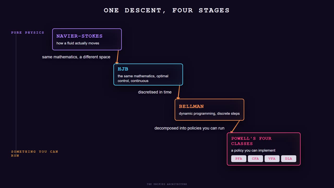
One more chain to record before the argument moves on, because it connects both halves of the entry so far. Navier-Stokes describes physical flow. HJB is the same mathematics governing flow through a space of possibilities. Bellman is HJB discretised in time. Powell's four classes are the Bellman framework decomposed into things you can implement. Goertzel's reading adds the regime layer on top: the Reynolds number of a decision problem indicates which class is appropriate, with cheap direct policies suiting the laminar case and expensive simulation earning its cost only when the environment turns turbulent. Four levels of description, one object, and each level hands the next one something it can build with.
What a property graph cannot say
A decision layer needs something to decide over. The four policy classes all assume a representation of the world is available, and the quality of that representation puts a hard ceiling on the quality of any policy running above it. This section is about a specific ceiling in the representation almost everyone reaches for first.
The graph you already know
If you have used Neo4j or any graph database, the property graph model is already intuitive. Nodes are entities: companies, tools, people, concepts. Edges are typed relationships: USES, COMPETES_WITH, DEPENDS_ON. Both carry properties as key-value pairs: timestamps, confidence scores, descriptions.
What makes this more than a database is that the shape carries meaning. Asking what a given system depends on traverses a web of typed connections rather than joining tables, and the topology itself (what clusters, what bridges, what has unusually many inbound edges) is information no relational schema exposes. The state-machine entry makes the parallel argument for modelling work this way rather than as a list of statuses.
The ceiling, stated precisely
An edge in a property graph connects exactly two nodes. You can hang properties on it, and those properties are flat values. An edge cannot point at another edge, which means a statement about a relationship has no native home in the model.
That sounds like an edge case until you notice how much real knowledge has that shape. Who asserted this relationship. How confident we are that it holds. Which other relationships fail if this one does. When it stopped being true. Every one of those is a fact whose subject is a relationship rather than a thing, and each one has to be either flattened into a property that cannot reference anything, or faked with scaffolding.
Four rungs, one capability each
The progression to the frontier has four steps, and each adds exactly one structural capability.
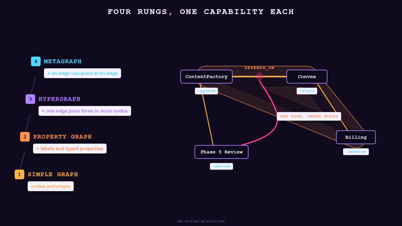
simple graph     pairs of nodes joined by untyped edges
property graph   + labels, types, flat key-value properties
hypergraph       + one edge may connect any number of nodes
metagraph        + edges that target edges, vertices that contain subgraphs

formally:  MG = (V, MV, E, ME)
  V   ordinary vertices
  MV  metavertices, each containing a subgraph
  E   ordinary edges
  ME  metaedges, connecting edges to edges or to metavertices
The hypergraph step is the one people meet first, and it fixes a real problem: a meeting involving five people is one relationship among five participants rather than ten pairwise edges that lose the fact they belong together. The metagraph takes both remaining extensions at once.
Two properties separate the top rung from everything below it. Metavertices are holonic, after Koestler's holon: a thing that is simultaneously a whole and a part. A metavertex for a company can contain its entire internal graph of dependencies, people and pipelines, while being one node inside a larger structure. Zoom in and the internal structure is there; zoom out and it is a dot, with no copy and no second representation to keep in sync.
A map analogy carries the difference well. A knowledge graph is cities connected by highways. A metagraph also shows regions, where an entire area with its internal roads is one navigable unit, and it shows commentary on the roads themselves: the budget that funded this highway, the traffic report saying it is congested, the rail line competing for the same route. The road participates in relationships rather than only connecting the cities at its ends.
A concrete thing you cannot say
Start from a relationship anyone would store: one system depends on another. Now add what an operator actually knows about it. This dependency was identified by a specific architecture review, it carries a criticality rating, and if it breaks, three other units are affected.
A property graph gives you two options and both cost something. Flatten it: add criticality: "high" and identified_by: "phase5_review" as properties on the edge. The rating survives and the impact claim does not, because a property cannot point at the other relationships that would fail. Or scaffold it: create a dependency-assessment node joined to both entities and to the downstream ones. That works, and it puts an object in your graph that no one in the business would recognise, because it represents nothing in the world. It exists to route around the model.
In a metagraph the dependency edge is itself an entity other edges can target, so the review points at the relationship and the relationship points at the relationships it would take down with it. No invented nodes, and the stored structure matches the sentence a person would say out loud.
Reification, and why the workaround feels forced
This problem is old and has a name. In RDF and OWL the pattern is called reification: to make a statement about a statement, mint an intermediate resource standing for the statement and attach properties to that. It works, it is standard, and it has been quietly irritating semantic web practitioners for two decades, because the intermediate resource is an artifact of the encoding rather than a part of the domain. A metagraph makes reification native instead of a bolt-on, which is the same amount of expressiveness with the scaffolding removed from view.
Self-reference is the real prize
The capability that matters most comes from pointing the structure at itself. A metagraph can hold nodes representing the set of all high-criticality dependencies, edges connecting a known gap to the query that would fill it, and metavertices containing everything the system knows about its own uncertainty. Those are statements about the graph, living in the graph, queryable by whatever queries the domain knowledge.
This is the line where a store stops being a database and becomes a world model. A database holds what you know. A world model also holds what you do not know, how confident you are about where that boundary sits, and what you would have to observe to move it. Every retrieval system that ends up confidently answering a question it had no business answering is a system with the first thing and without the second.
The retrieval consequences are direct, and the retrieval entry works them through in practice. The next section takes the other route into the same territory: a system built on this substrate deliberately, and four tools that turn out to have been building one without saying so.
The metagraph, and four tools already building one
An argument that a structure is necessary is worth more when someone has built on it. Two pieces of evidence follow: a research system that chose the metagraph deliberately and says why, and a set of ordinary production tools that arrived at pieces of the same shape without meaning to.
A system that chose it deliberately
Ben Goertzel selected metagraphs as the core data structure for OpenCog Hyperon, and the stated reason is the capability from the end of the last section rather than elegance: a knowledge graph cannot represent a system reasoning about its own reasoning. A graph can store the fact that a clustering method organises documents hierarchically. A metagraph can store that fact, the inference that produced it, the confidence attached to that inference, and the alternatives considered and rejected, in one structure under one set of operations.
The formal version of the argument is in Goertzel's paper on reflective metagraph rewriting, whose claim is that intelligence requires a substrate supporting self-modification: the system has to be able to treat its own knowledge, its own inference rules and its own learning procedures as data, alter them, and observe what happens. Ordinary graphs lack both the recursion and the reflexivity that requires.
The Atomspace is the implementation, a distributed in-memory store built from immutable typed Atoms. Links connect any number of atoms, and atoms can themselves be links, which is the metaedge property arriving as a basic fact about the type system rather than as a feature.
A calibration belongs here, since this entry keeps insisting on stating things at their real strength. Hyperon is a research system in active pre-alpha development rather than proven production infrastructure, sitting at version 0.2.10 as of early 2026. It is an existence proof that the structure can be built and reasoned with, and it is not evidence that a metagraph is the right store for your application this quarter. Both halves of that sentence matter to the argument.
Confidence and attention as first-class properties
Every atom in that store carries two values a property graph cannot represent as first-class objects. A TruthValue is a probabilistic confidence measure saying how much to trust the item. An AttentionValue is a resource-allocation weight saying how much computation to spend on it.
Their power is that the system can reason over them directly. This fact has low confidence and low attention, so it is both uncertain and neglected, which makes it a candidate for investigation. That is a sentence about the state of the knowledge base, expressible in the same language as any sentence about the domain. An attention weight sitting in the same structure as the knowledge it points at is the memory-side version of the Reynolds dial, a resource allocation computed from the state of the system rather than configured in advance.
When the program is the same substance as the data
Hyperon's language, MeTTa, is built so that programs are themselves metagraph structures. Running one means applying rewrite rules to the metagraph: match a pattern, replace it, observe the result.
Four levels then live in one place with no partitions between them. A fact. A rule that operates on facts. A meta-rule governing when rules fire. And the application of the meta-rule to the rule. There is no separate rule engine and no meta-reasoning module attached to the side, which is the structural payoff of the whole chapter: the boundary between knowledge and the process that operates on knowledge dissolves, and anything the system can do to the world model it can also do to itself.
One further design property is worth carrying because it recurs later in this entry at organisational scale. In Hyperon's architecture, multiple subsystems share the memory and no single subsystem can access the entire global state. Each is a bounded internal observer, building a model of the whole from the part it can see, and each is also represented as data inside the same store, so it can query its own representation to explain its own failure. That constraint is the same one every distributed system and every team of agents lives under, and it is the seed of the argument about bounded observers that returns when the market shows up.
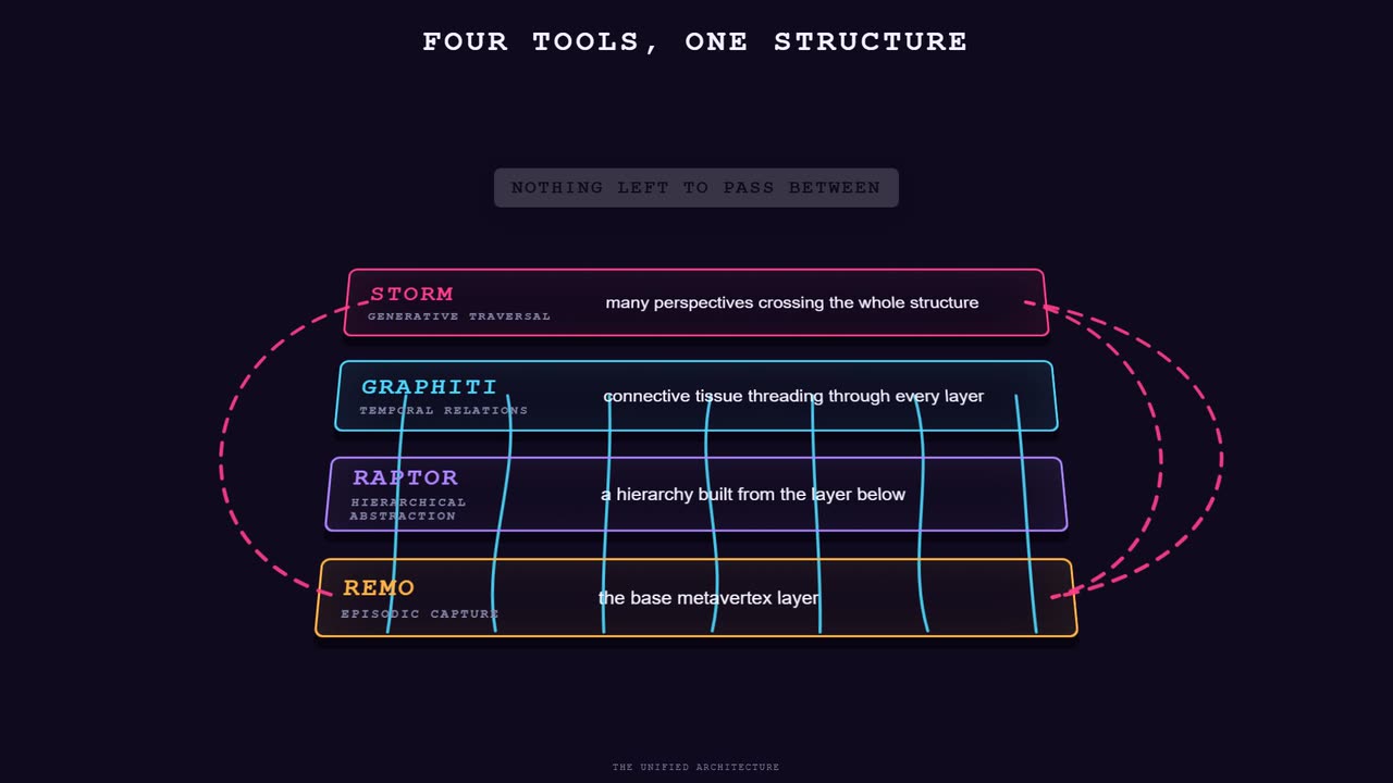
Four tools, four altitudes
Now the accidental evidence. A working knowledge stack tends to accumulate four tools doing four jobs, bought or built separately, wired together with adapters. Read as one structure rather than four systems, they line up as altitudes of a single recursive graph.
| LAYER | WHAT THE TOOL DOES | WHAT IT IS IN METAGRAPH TERMS |
|---|---|---|
| Episodic capture REMO | records every interaction as a timestamped episode, then rolls raw episodes up into summaries | the base metavertex layer. rolling summarisation is literally the operation of building higher metavertices from lower ones. |
| Hierarchical abstraction RAPTOR | clusters chunks, summarises each cluster, clusters the summaries, repeats to the top | a metavertex hierarchy. retrieval at a chosen altitude is navigation to a depth rather than a different index. |
| Relational tissue Graphiti | tracks entities and typed relations across episodes and across time, with validity windows | the metaedge layer. a fact with a valid-from and valid-until is an edge carrying its own lifecycle. |
| Generative traversal STORM | simulates multiple expert perspectives interrogating the corpus, then synthesises | a traversal pattern entering from several points at once. each perspective is a corridor, and synthesis happens where corridors cross. |
Held that way, capture, organise, connect and generate stop being pipeline stages that hand artifacts along. They become concurrent operations on different aspects of one structure, each modifying what the others read.
What a temporal graph already gets right
The distance to close is shorter than the formalism suggests, because a well-built temporal knowledge graph has already grown proto-versions of every metagraph feature. Validity windows on facts treat relationships as objects with lifecycles, which is most of the way to a metaedge without the ability to target one. Episodes function as handles for subgraphs, which is a metavertex without formal containment. Community detection identifies which nodes belong together, producing labels where a metagraph would produce containers. Namespace isolation draws boundaries around subsets, which is containment kept flat.
None of that convergence was aimed at metagraph theory. It happened because temporal tracking, episodic memory, emergent grouping and namespace isolation are the problems that motivated metagraph theory in the first place, so anyone who takes those problems seriously walks toward the same structure from the other end.
Database, memory, operating system
property graph            facts and relationships                      a database
temporal knowledge graph  + how they evolved and when                  a memory
metagraph                 + hierarchy, self-reference, and the
                          processes that operate on all of it   an operating system
There is a second reading of that top rung worth recording, because it connects this chapter to how the systems in the back half of this entry are actually built. An entity component system, where an entity is a bare identity, components are data attached to it, and systems are functions operating over everything carrying a given component, is the same architecture described computationally rather than structurally. An entity is a metavertex, a component is a property set on it, and a system is a traversal pattern. Noticing that saves you from designing a bespoke structure every time the same problem shows up wearing different clothes, which is the practical form of everything this entry has argued so far.
The path from a working temporal graph to a metagraph is incremental, which is the useful conclusion. Formalise episodes as containers. Add edge-to-edge references. Implement hierarchical containment. Build the self-referential layer where structural properties of the graph become nodes in it. Connect the abstraction tree to the metavertex hierarchy as a view rather than a copy. Every step is independently useful, which means none of it requires believing the whole argument before starting.
Three chapters have now built a foundation: the mathematics, the decision layer, the knowledge structure. What follows is the part where all three meet a domain that does not care about any of them.
Seven sins, one false assumption
Three chapters of foundation now meet a domain that has no interest in any of it. Quantitative finance is the right proving ground precisely because it is adversarial, it keeps score in a currency nobody can argue with, and it has a large, sophisticated, well-funded literature that keeps making the same small number of mistakes.
The assumption nobody writes down
There is a claim at the centre of nearly every backtesting framework, every published strategy and most institutional risk models, and it survives because stating it plainly is embarrassing. The claim is that markets are stationary.
Nobody writes "we hereby assume stationarity" in their documentation. They do not have to, because it is load-bearing by default. Compute a historical Sharpe ratio and present it as a performance metric, and you have assumed the distribution that produced it continues to operate. Fit on a training window, apply to a test window, and skip the question of whether the regime changed between them, and you have assumed it again. Compute a value-at-risk figure on a fixed lookback volatility estimate, same assumption. Run a unit-root test, reject, and proceed as though the distributional structure is now understood, and you have skipped the harder questions: stationary relative to what window, over what regime, conditional on what state of the surrounding system.
A stationary process has constant mean, constant variance and constant autocovariance structure across time. Name one financial asset that satisfies that definition over any meaningful horizon. Take your time.
Three kinds of non-stationarity
The failure has three distinct shapes, and separating them matters because each one breaks a different part of a system. All three exist in equities. Crypto makes each categorically worse rather than incrementally worse, which is a claim about kind rather than degree and is worth defending row by row.
| TYPE | WHAT MOVES | EQUITIES | CRYPTO |
|---|---|---|---|
| Distributional | the return distribution itself, and the correlations between assets | regime shifts on quarterly to annual timescales. the run into the 2008 crisis unfolded over roughly 18 months of deteriorating credit before the acute phase. | days to weeks. Correlation structures themselves shift with volatility regime, so portfolio risk models calibrated in one regime are wrong in the next. |
| Structural | the data-generating process, including which assets exist at all | decadal. floor trading to electronic markets, then the rise of passive indexing. slow enough for adaptive models to track. | continuous. the tradeable universe reconstructs itself monthly, and over 80% of 2025 token launches traded below their listing price. that is the base rate rather than a tail. |
| Reflexive | how fast a shift propagates before anyone can respond | circuit breakers halt trading at defined decline thresholds, interrupting cascades and letting participants update. | continuous trading with no halts. futures-spot relationships shifted instantly on the November 2024 US election result, with nothing to buffer the transition. |
The reflexive row deserves the fluid reading, because it is the one the framing from earlier explains best. A circuit breaker is a viscosity injection. It adds friction precisely when inertia is running away with the system, which is the mechanism that keeps a flow from going fully turbulent. A market without halts has removed the damping term from its own equation, so a regime shift that takes hours elsewhere takes minutes there, and any system requiring batch recalibration is structurally too slow to participate in its own defence.
Supply mechanics add a second structural amplifier with no equity parallel. Airdrop distributions deliver instantaneous sell pressure from holders with zero cost basis, which alters order flow for weeks. Copula analysis of stablecoin flows finds that stablecoin accumulation and activity Granger-cause crypto volatility. None of that is exotic once you accept the framing. It is external forcing, the fourth term in the equation from the water-in-a-pipe section, arriving at a cadence the model was never fitted to.
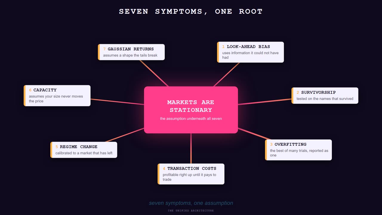
The seven, named precisely
Naming them exactly is the prerequisite for the next section, where each one gets matched to a specific structural mechanism. The order is the conventional one and roughly tracks how early in a project each tends to appear.
| SIN | WHAT IT IS, AND THE SUBTLE FORM PEOPLE MISS |
|---|---|
| 1. Look-ahead bias | using information the system could not have had at execution. The obvious form is trading on a close you only learn after the close. The subtle form hides in normalised features: a rolling z-score computed over a window that includes the current observation lets every point normalise itself against a distribution containing itself, so the signal knows the future because the future is in the denominator. |
| 2. Survivorship bias | testing on an asset universe defined by what is still alive today. A backtest on current index constituents silently excludes everything that failed, and in crypto it excludes every rug, every abandoned project and every token trading at a thousandth of its peak. The live system had no way to know which names to exclude in advance. |
| 3. Overfitting | testing many parameter combinations and reporting the best. Bailey, Borwein, Lopez de Prado and Zhu showed the probability of selecting an overfit strategy rises rapidly with the number of trials, and that memory effects in financial series make overfitted strategies systematically underperform out of sample rather than merely fail to outperform. The deflated Sharpe ratio exists to adjust a reported Sharpe for the number of trials, the skew and the kurtosis behind it. |
| 4. Transaction cost fantasy | a strategy that is profitable before costs is a cost-estimation exercise with a sign error. In microcap market making, where the spread captured per level and the fees paid per side are the same order of magnitude, costs are the primary variable deciding the sign of the result rather than a perturbation applied to it. |
| 5. Regime ignorance | the most consequential one. A strategy calibrated to a ranging market and deployed into a trending one actively loses money rather than underperforming: it fills on the wrong side of the move, accumulates against a sustained trend, and stops out at maximum distance from entry. Practitioners with years of live systematic trading name it among the most consistent causes of backtest-to-live collapse. |
| 6. Capacity delusion | every backtest assumes the strategy takes prices rather than makes them. Past some size relative to daily volume, entries and exits move the market against you, and the system is setting a price while its model still assumes it is discovering one. The backtest becomes a forecast for a place the forecaster has left. |
| 7. Distribution assumption failure | classical models assume returns come from a parametric family, usually Gaussian. Real returns are fat-tailed, skewed and serially correlated. A 2025 paper modelling markets with fluid-dynamics machinery argues the reason is structural: flows concentrate and diffuse, pressure builds unevenly, and disturbances propagate, which is turbulent behaviour rather than Gaussian noise. |
Run the trace and all seven arrive at the same root. Look-ahead and survivorship assume the sample represents the future. Overfitting assumes a pattern found in one sample persists. Cost fantasy assumes friction is stable enough to subtract later. Regime ignorance assumes the calibration still applies. Capacity assumes your presence does not change the system. Gaussian assumes the shape of the distribution holds. Six of the seven are stationarity wearing different clothes, and the seventh, capacity, is the special case where the thing breaking stationarity is you.
That is why patching them individually keeps failing. Each patch addresses a symptom of one assumption while leaving the assumption in place, which is how an industry accumulates seven separate literatures for one problem. The section after next takes the alternative route: change the structure so that each sin has nowhere to live.
Why an industry that knows better leaves it alone
A list of seven well-documented errors raises an obvious question. These are not obscure. Every one of them has a literature, a name and a standard countermeasure. So why does an industry full of genuinely brilliant people keep shipping models that carry them?
The explanation is incentive structure
Start by discarding the comfortable answer. The people building institutional models are highly capable, frequently more mathematically sophisticated than the people criticising them, and entirely aware that markets move. The failure is produced by what the surrounding system rewards.
Consider what a career actually optimises for. A model gets built across many months. It is reviewed by a committee, which generates revisions, which are reviewed by another committee. At no point in that sequence does anyone benefit from asking what happens if the regime changes, because that question implies the work needs reconsidering and is professionally inconvenient for everyone in the room. The result passes review. Whether it survives contact with a market it was not fitted to is a question that arrives long after the approval, attributed to conditions nobody could have foreseen.
A word used as a period
There is a verbal tell for this, and it is worth naming because once you hear it you cannot stop. The word "robust", deployed as a complete thought. As in: we need to ensure the model is robust. Full stop. No specification of what it is being made resistant to, over what distribution of shocks, relative to which alternative. The word signals guild membership while communicating nothing, and it functions as a way to close a conversation about model risk without having one.
The same move shows up in how the seven sins get discussed inside institutions, where they become "known challenges in the literature". That phrasing is the professional equivalent of noting that the building has no fire exits, that this is a recognised architectural challenge, and that there is a paper about it.
What the surrounding system actually rewards
| MECHANISM | WHAT IT REWARDS | WHAT IT LEAVES UNREWARDED |
|---|---|---|
| Basel III and IV, FRTB | internal models that clear regulatory thresholds, or standardised approaches that avoid the question | predictive accuracy against conditions absent from the reference data |
| Attribution tests and non-modellable risk factor penalties | models shaped to pass the test and avoid the penalty | novelty, since an unusual factor is expensive to carry regardless of whether it is correct |
| The standard two-and-twenty fee structure | growth in assets under management, and concentrated bets that pay in good years | consistency that compounds, since the manager holds the upside without proportional downside |
Read the third column as a set.
A different selection pressure
Set that against an operator whose own capital is in the position. There is no committee, no validation period, and no buffer. The model ships, the market responds, and the feedback arrives in hours with the operator's own money attached to it.
That symmetry produces a different relationship with model uncertainty, and it is worth being precise about why. Someone who has watched a strategy generate consistent returns for six weeks and then give it all back in four hours, because the market went from ranging to trending on a catalyst their signal stack did not anticipate, has learned something about regime change that no amount of reading produces. The lesson is a shorter loop between being wrong and finding out. Every architectural choice in the next section is downstream of trying to make that loop shorter still.
The pattern is symmetric across both worlds, which is what makes it structural rather than tribal. Correlation parameters calibrated during a benign regime failed to capture correlated defaults in 2008. Momentum behaviour carried over from a prior cycle herded capital into failing assets in 2022. Same error, different decade, different asset class, different professional culture.
Fifty years of evidence, almost entirely undeployed
The last part of the indictment is the strangest, because the tools have existed for half a century.
Benoit Mandelbrot connected turbulence theory to financial markets in the 1960s and 1970s, drawing on Kolmogorov's 1962 model of turbulence intermittency. The structural insight is the cascade from earlier in this entry: energy passes from large scales to small through a multiplicative random process, distributing unevenly at each scale, producing bursts of intense activity separated by relative calm. Mandelbrot observed that financial returns carry the same multiscale, bursty, intermittent structure.
The formal version is quantitative rather than impressionistic. A monofractal process such as Brownian motion has the same statistical structure at every scale. A multifractal process has different structure at different scales, and the parameter measuring the curvature of the scaling exponent function is non-zero in both turbulent velocity data and financial time series. Both are multifractal, measured the same way, by the same statistic. That is a testable claim rather than a resemblance, and it has been tested repeatedly for fifty years.
The landmark result is Ghashghaie and colleagues in Nature, 1996, showing that the distribution of foreign exchange rate changes across time scales follows the same cascade structure as velocity differences across spatial scales in turbulent flow. Mantegna and Stanley found power-law scaling behaviour in the S&P 500. Bouchaud extended multifractal cascade modelling to volatility intermittency and endogenous market dynamics. The school's conclusion is that the shared statistical properties are the same scaling relations, the same cascade structure and the same intermittency patterns, with capital flow standing where molecular velocity stands and transaction costs standing where molecular friction stands.
And the deployment of that work in active trading is close to zero, confined to academic groups and a small number of firms such as Capital Fund Management, which has worked in this tradition since the early 1990s. Fifty years of validated science, a handful of practitioners, and an assumption everyone knows is false still sitting under the standard toolkit. That gap is the argument for the next section, and it is also the reason the argument is available to anyone willing to read the papers.
Dissolved rather than solved
An enumeration of known problems with no structural answer is a genre, and quantitative finance has a large shelf of it. What makes the next argument different is the claim that each of the seven has a mechanism that makes committing it impossible, rather than a practice that makes committing it less likely.
The architecture in compact form
Goertzel's FluQNet, meaning fluidic quantum neural networks, takes the triangle from the first third of this entry and turns it into a computational framework on one core move: treat computational activity as a conserved fluid flowing through a network, routed without being created or destroyed.
That conservation is doing real work rather than adding flavour. Total attention in the system is fixed, so routing it toward one part necessarily withdraws it from another. That is the incompressibility condition, and it is exactly what licenses the Navier-Stokes machinery from the theorem section. A system that can simply allocate more attention everywhere is not a fluid and gets none of the results.
Two coupled layers sit on top of it. A classical routing layer moves computational budget through the network graph under the fluid dynamics, with pressure gradients drawing resources toward nodes that need them and viscosity preventing resources from sloshing between nodes faster than is useful. A quantum operator layer handles local inference, where each node holds a density matrix rather than a scalar activation, so a node can carry a genuinely mixed state instead of committing to one value.
The connection between them is the framework's central technical claim. Both layers are formalised as functors from the network's free path category into vector spaces, and the requirement is that natural transformations between them commute on every edge, which then makes them commute on every path. Stated without the category theory: moving budget from one node to another and performing inference from one node to another are two descriptions of the same operation, and the architecture forces them to agree.
What falls out when that constraint is enforced is the part worth remembering. Traffic concentrates on paths where the two layers align most easily, and those high-use paths become semantic corridors: routes that are simultaneously cheap to move resources along and coherent to reason along. They form the way rivers carve canyons, from repeated use rather than from design, which is the same self-organising behaviour the knowledge chapter predicted for frequently traversed query paths.

Seven sins, seven structural mechanisms
Here is the mapping in full, which is the densest single object in this entry. Each row pairs a failure mode from two sections back with the specific structure that removes it.
| SIN | STRUCTURAL MECHANISM | WHY THE SIN HAS NOWHERE TO LIVE |
|---|---|---|
| 1. Look-ahead | predictive coding, strictly forward-only information flow | no mechanism exists in the computational graph for future information to reach a past parameter. every signal is indexed to the information state at its own timestamp. |
| 2. Survivorship | metagraph lifecycle encoding | dead assets are labelled terminal with full trajectory preserved as navigable structure. nothing is deleted, so nothing can be silently excluded. |
| 3. Overfitting | the corridor compatibility kernel, positive semidefinite by construction | complexity is bounded by a mathematical property of the object rather than by a penalty term someone chose. you cannot posit more corridors than the market has without breaking the constraint. |
| 4. Cost fantasy | viscosity as a primary term in the governing equations | friction enters before the optimisation rather than after it, so what comes out is a different configuration rather than the frictionless one with a haircut. |
| 5. Regime ignorance | a Reynolds-style ratio with thresholds adapted from live prediction error | the regime is a continuously updated reading rather than a label assigned by a model fitted to regimes that have ended. |
| 6. Capacity | the passive tracer constraint, monitored through own-fill impact | the condition is stated on the system's measured effect on the flow rather than on a size assumed safe before deployment. |
| 7. Distribution failure | density-matrix state representation | no parametric family is assumed at all, and genuine ambiguity between regimes is representable instead of being forced into a single classical choice. |
A guardrail rather than a sign
The first row carries a distinction that generalises to the whole table, so it is worth slowing down on. Classical backtesting frameworks are vulnerable to look-ahead because nothing in their architecture prevents the leak. The protection is a discipline held by a person, and people ship things late on a Friday.
Predictive coding removes the possibility rather than the temptation. Each node generates a prediction about the next state from its current state and history alone, then receives a correction once the actual outcome arrives. Information flow is causal and forward-only, implementing Karl Friston's free energy principle, where the system reduces surprise by minimising prediction error across a hierarchy. No current-period statistic can normalise itself against a distribution containing itself, because the machinery to reach backwards does not exist.
Think of it as the difference between a guardrail and a sign. A sign says do not drive off the cliff. A guardrail makes driving off the cliff physically impossible. Every row in the table above is an attempt to replace a sign with a guardrail, and the value of the distinction is that a guardrail does not degrade when the person watching it gets tired.

The graveyard is the training set
The survivorship row inverts the usual handling in a way worth stating on its own. Classical treatment discards dead assets, which is what produces the bias. The metagraph model labels them terminal and keeps the full trajectory as navigable structure, so when a live asset starts exhibiting the signature that preceded a historical failure, the evidence from every prior instance of that signature is available at the moment it is needed.
That converts survivorship bias from a data problem into a data asset. The most informative thing about a failed asset is exactly when and how it failed, and that is precisely the information a live position needs. The parallel is epidemiological. You do not study only the patients who recovered, because the factors distinguishing recovery from death are the factors that matter for treatment, and a sample with the dead removed produces a model that cannot predict death.

Friction changes the shape of the answer
The cost row makes a claim stronger than it first sounds, and the fluid mechanics is what backs it. Viscosity in the Navier-Stokes equations does more than remove energy from a flow. It redistributes energy across scales, suppresses small-scale turbulence, and creates boundary layers near surfaces. Drop it and you get physically nonsensical results, including infinite velocities at a wall.
The same holds for a strategy. Computing the optimal configuration with costs present produces different spacing, a different range and a different allocation, rather than the frictionless configuration with a deduction applied. The optimal thing to do in the presence of friction is a different thing, not the same thing done less profitably.
Two specific structures follow, and both are borrowed with their arithmetic intact. The Kolmogorov microscale, which in turbulence is the smallest eddy size where viscous dissipation overwhelms inertia, has a direct market analogue: a minimum spacing below which the cost of acting at that scale exceeds the value available at that scale. Below the floor, nothing is profitable regardless of how much structure exists at larger scales, and the threshold is computed from the friction coefficient and the local volatility rather than discovered by paying for it. And no-trade zones behave as boundary layers whose thickness is set by local order book depth: a thin book means high friction, a thick boundary layer and small effective capture, while a deep book approaches the theoretical value. Higher viscosity also moves the regime boundaries themselves, so a high-friction venue needs more turbulence before the same strategy becomes viable there at all.
A regime that is felt rather than classified
The regime row contains the sharpest mechanical difference between this design and a conventional one. A classical classifier has fixed thresholds fitted to historical data, which makes it stationary by construction and guarantees failure exactly when boundaries move.
The alternative deploys a configuration based on its current estimate, observes whether the world responds as predicted, and updates the boundary estimate from the error. Regime change gets detected through the accumulation of systematic prediction errors, meaning errors that all point the same way rather than scattering, which is a different signal from simply being wrong. The regime is continuously felt and adapted to rather than classified and then acted upon, and the difference shows up precisely in the transitional band where a classifier has to commit to a label that is about to stop being true.
Stay a leaf
The capacity row supplies the precise condition that a size limit only approximates. A system is a passive tracer when its deployment does not measurably alter the pressure gradient: a leaf on a river moves with the flow without changing it, and a boulder changes the current. The requirement is to remain a leaf.

Operationally that becomes a measurement rather than an assumption. The system watches its own fill impact, comparing the mid-price when an order was placed against the mid-price when it filled, corrected for market movement it did not cause. A consistently non-zero and directional impact, where buying pushes price up and selling pushes it down, means the threshold has been crossed. A share-of-volume ceiling is the coarse constraint; the fill-impact monitor is the live one, and it works without a pre-deployment capacity study built on data that has aged.
The same reasoning bounds the operating band from both directions. Too little liquidity and even small positions move the market, so friction is too high to be a tracer at any size. Too much and institutional operators are competing for the same spread with better infrastructure, which compresses what is available. The workable band sits between those two walls, and its location is derived from the tracer condition rather than picked.
Why quantum formalism, for a market that is not quantum
The last row is the one most likely to trigger a reasonable allergy, so it needs its argument stated carefully. Nothing here claims markets are quantum mechanical. The claim is about the observer.
A regime detector is a bounded observer of a large classical system. It cannot see the true microstate, meaning every order, every holder and every latent intention, and it receives instead a coarse, delayed, filtered stream: price, volume, book depth, funding. Goertzel's argument runs through four levels of what he calls quantumity that emerge under exactly those conditions. Opacity forces coarse-graining into equivalence classes. The order in which you query matters, which makes observations noncommutative. Subsystems become correlated in ways that mirror entanglement. And under pragmatic closure the observer's own statistics can violate Bell-type inequalities.
So the quantum formalism is the control-optimal description available to a bounded observer of a complicated classical system, rather than a claim about the system's underlying physics. Classical probability turns out to be the special case that applies when the compatibility structure is diagonal, which in a volatile market it rarely is. That framing is worth holding because it is the same bounded-observer constraint from the metagraph chapter, where no subsystem could see the global state, arriving now with a quantitative consequence attached.
Which brings the chapter to its actual claim. The problems are dissolved rather than solved, and the distinction carries weight. A solved problem returns when the solution stops being maintained. A dissolved problem cannot return, because the foundation that allowed it is gone. Walk-forward validation, purged cross-validation and regime-conditional testing are all genuine improvements, and each one is a better sign. None of them is a guardrail.
One caution to carry out of this section, in the spirit of the calibration made when the theorem was introduced. The mathematical results underneath these mechanisms are published and checkable. The integrated system built from them is a design rather than a track record, and any architecture that has dissolved a problem on paper still has to survive contact with the thing it was designed against. What the next chapter argues is that the shape of that architecture keeps appearing in places that have nothing to do with markets, which is a different kind of evidence that it is the right shape.
Everything converged on a compiler
Five sections of foundation now have to answer an operational question. If all of this is one structure, what does a system built to treat it that way actually look like? The answer turned out to be a pattern so old that most engineers stopped seeing it years ago.
Why compiler phases run in that order
A compiler turns source text into machine instructions through a sequence of phases, each taking the previous phase's output, transforming it, validating the result and passing it on. The ordering is forced rather than chosen. You cannot optimise code that has not been parsed, and you cannot parse tokens that have not been lexed.
What makes the ordering interesting is the property underneath it. Each phase narrows the space of valid artifacts, so every later phase inherits guarantees rather than obligations. Raw characters can be anything. Tokens have to be valid lexemes. The syntax tree has to be grammatically valid. The typed tree has to be semantically valid. The optimised intermediate representation has to mean the same thing the original meant. At each boundary a quality gate eliminates an entire class of defect, which is precisely why downstream phases can be simple: they were built knowing what can no longer reach them.
raw text  →  lexer  →  parser  →  semantic analysis  →  optimisation passes  →  codegen  →  linker
            |          |              |                       |                     |
          invalid    grammar         type and scope           IR verifier         unresolved
          lexeme     violation       error                    per pass            symbol

each gate deletes a class of defect. nothing downstream has to handle it again.
The optimisation stage is the instructive one. LLVM runs dozens to hundreds of small passes rather than one large one, each targeting a specific inefficiency, each independently testable, each taking valid intermediate representation in and producing valid intermediate representation out, with a verifier between them confirming the transformation preserved meaning. Many small verified passes reach an optimisation level no monolithic pass achieves, because each one works inside a tractable scope while inheriting every previous pass's cleanup.
And GCC's pipeline adds the property that turns a sequence into a system. Profile-guided optimisation compiles with instrumentation, runs the program, collects an execution profile, then recompiles using it. Execution data from one cycle improves the next cycle, which is the compounding loop that shows up in every pipeline in the rest of this entry.
Three pipelines that arrived at the same shape
Three production systems I run have nothing in common at the domain level: one produces software, one produces written work, one produces trades. Each was built at a different time for a different purpose, and each independently grew the same skeleton.
Code. Requirements analysis decomposes a problem statement into discrete requirements. A spec structures those into an architecture with acceptance criteria. Implementation produces the code. Then the gates fire in sequence: lint for syntax and formatting, property-based tests for behaviour across all valid inputs, an observability check confirming every function doing I/O carries instrumentation, an architecture check for functional style and typed models, and a human review for the strategic judgment no deterministic gate can supply. Merge resolves the branch against the trunk.
Written work. Demand and landscape research narrow an open topic into a defined one. Gap analysis and competitive reading structure it. Drafting happens incrementally against a hard per-pass word ceiling, for the reason given at the very top of this entry: quality degrades measurably in a single long generation. Then separate optimisation passes run, each targeting one class of defect: coverage gaps, structural and flow problems, formatting, and a final pass for the cross-domain connections that give the work its character. Linking connects the output into the surrounding corpus, which is the same job a linker does.
Trading. Market data ingestion cleans raw ticks into bars. Feature engineering derives indicators. Regime detection classifies the state. Strategy selection proposes parameters for that state. Aggregation weighs multiple proposals. Then the gates: hard numeric risk checks, simulation across many price paths, portfolio-level exposure limits. Only a configuration that clears all three reaches execution, and post-trade analysis feeds the next cycle, which is profile-guided optimisation wearing different clothes.
The operating rule from the trading system's own documentation is the whole pattern compressed: "LLM recommendations never bypass hard numeric risk checks. The math layer has veto power. Creativity sits upstream of gates, not downstream." Generative components propose. Deterministic components decide what executes. Once that boundary is drawn, you can let the creative half be as adventurous as you like, because the expensive failures are on the other side of a wall it cannot reach through.
The mapping, part for part
Held against each other at the right altitude, the three stop being similar and become the same pipeline with different payloads.
| COMPILER PHASE | CODE PIPELINE | CONTENT PIPELINE | TRADING PIPELINE |
|---|---|---|---|
| Preprocessor | dependency resolution, environment setup | ingestion. normalise formats, extract text, expand references | tick data cleaned into bars |
| Lexer | requirements broken into discrete units | entity and keyword extraction from raw source | feature engineering into indicators |
| Parser | the spec. structure plus acceptance criteria | concept mapping into a knowledge tree | structural read of the current market state |
| Semantic analysis | type checks, architecture compliance | alignment check. does this trace to a real objective | regime detection |
| Optimisation passes | refactor, lint, property tests | coverage, structure, formatting, voice, each its own pass | proposal aggregation and parameter refinement |
| Verifier between passes | tests still green, lint clean | deterministic detectors. the em dash gate is one | numeric risk checks with veto power |
| Code generation | implementation against the spec | drafting, capped per pass | the frozen configuration sent to execution |
| Linker | merge, resolve symbols against the trunk | internal linking and citation into the corpus | portfolio-level exposure reconciliation |
| Standard library | shared packages | the skills library, callable by any run | shared strategy and risk primitives |
| Profile-guided optimisation | production telemetry driving the next refactor | research graphs and performance data feeding the next piece | post-trade analysis tuning the next cycle |
Five properties that hold across all three
Stripping the domains away leaves five structural properties, and they are the portable part. Anything with all five behaves like a compiler whether or not anyone involved has used the word.
| PROPERTY | WHY IT IS LOAD-BEARING |
|---|---|
| 1. raw, unstructured, possibly invalid input enters | the system is designed for the input it will actually receive rather than the input it wishes for |
| 2. sequential refinement passes, each depending on the last | each pass stays small enough to be correct, and inherits the cleanup of everything before it |
| 3. deterministic gates between passes | a gate takes an artifact and returns pass or fail with no judgment involved, so it never gets tired and never negotiates |
| 4. creative work upstream, enforcement downstream | creative quality depends on whoever is doing the work; enforcement quality depends on gate definitions, which are reusable. this is the property that lets the system scale. |
| 5. every run produces data that improves the next run | without it you have a pipeline; with it you have a flywheel, where the output of each rotation is the input that makes the next one cheaper |
Property 4 is the one people skip, and skipping it produces a specific pathology. Push enforcement upstream into the creative phase and you get a system that produces safe, mediocre output, because the constraints are firing while the work is being invented. Leave enforcement out entirely and you get brilliant output that periodically destroys something. Separating them lets each half be maximally itself.
The same loop at three altitudes
The pattern is not confined to machines, which is the strongest evidence that it is structural. John Boyd's OODA loop, observe, orient, decide, act, was developed for air combat. Deming's PDCA cycle, plan, do, check, act, came out of manufacturing quality. They describe the same movement: read the current state, interpret it, act, and use the result to inform the next pass.
Every refinement pass in every pipeline above is one of these loops. Observe the current draft or intermediate representation or market state, orient to what is wrong with it, decide on a transformation, apply it. The loops then nest, which is the part worth rendering.
Toyota has a name for what the middle of that diagram requires. Jidoka is usually translated as automation with a human touch, and the split maps directly. The deterministic gates are the automation: they run identically every time and catch exactly the defect classes they were built for. Human review is the touch, catching what a deterministic check structurally cannot, which is strategic misalignment, voice drift, and a regime nobody has seen before. The andon principle completes it: any station can stop the line, and the line stays stopped until the cause is addressed rather than the symptom cleared.
The connection back to the mathematics is direct rather than decorative. Boyd's argument was that the pilot who cycles faster and more accurately than the opponent accumulates a compounding advantage, which is the Bellman equation stated operationally: the value of the current state depends on the quality of every decision that follows, so improving the loop improves everything downstream of it at once. OODA is Bellman made operational, PDCA is Bellman made industrial, and the compiler pipeline is Bellman made computational. Same recursion, three vocabularies.
One framework, many gate definitions
The operational payoff is what this buys when a new unit starts up. It needs three things rather than a bespoke operating model: a pipeline definition naming its refinement stages, gate definitions naming its deterministic checkpoints, and a feedback mechanism naming what telemetry improves the next cycle. Everything else is inherited.
Skills carry the shared procedures. Agents carry the domain-specific roles. Hooks enforce the universal gates regardless of domain, which is why a formatting detector fires on every write everywhere rather than per project. Teams provide the runtime coordination. And the lifecycle for building any new capability, from encoding a procedure to testing it to using it to wrapping it in a workflow to standardising it, is itself a refinement pipeline with gates, which makes it the pipeline for building pipelines.
The consequence that matters is the one about scarcity. The tools in this section are public, documented, and mostly free. What is rare is seeing that trading, writing and software production are the same architecture, and then building the thing that exploits the overlap instead of maintaining three separate operations that each rediscover the same lesson.
The factory floor
The architecture in the previous section runs, and this section is what running it looks like from the floor. The factory framing earns its place because the constraints turn out to be the same constraints, and manufacturing solved several of them decades ago.
Machines persist, operators rotate
Picture a floor with specialised machines. One cuts, one welds, one paints. Each has a fixed configuration, meaning tooling, calibration and safety interlocks, and that configuration survives the people who operate it. Whoever runs the machine today inherits the tooling installed last week.
An agentic development environment has the same two-part structure and most operational confusion comes from collapsing it. The machine is the configured environment: the loaded skills, the connected tooling, the project rules, the hooks. The operator is the specific agent instance that occupies it for one session. The machine keeps its configuration between sessions and between operators. The operator arrives, does work, contributes what it learned to shared memory, and disappears.
That separation is the reason the arrangement survives its own hardest constraint. Any single agent conversation is finite, and a long one degrades in ways the agent itself cannot detect, which is why every pass in this entry has a word ceiling on it. The machine has no such limit, because the machine is a configuration rather than a conversation. Design so that the durable knowledge lives in the machine and the ephemeral work lives in the operator, and session boundaries stop being a source of loss.
Assembly stations, and a pull system
On a physical floor, stations are separated so that work in progress at one does not corrupt output at another. Git worktrees give exactly that isolation: each lane works in its own directory on its own branch, the trunk stays clean, and parallel work generates no conflicts while it is in flight.
Coordination follows a pull pattern rather than a push one. Work sits in a queue, an agent claims an item when it has capacity, executes in its isolated station, passes the output through gates, and reports the result back to the queue. Work is pulled by available capacity rather than pushed by a central scheduler, which is Toyota's kanban logic and avoids the specific failure where a coordinator assigns six things to a crew that can hold two.
The asymmetry that decides where state belongs
One property of that arrangement drives more operational decisions than anything else on this list, and it is easy to discover the expensive way.
file-based state    project rules, local task lists, scratch files
                    copied into each station, never syncs back
                    station A cannot see station B's copy

cloud-based state   issue tracker, traces, knowledge graph, corpus
                    identical from every station
                    every operator, present and future, can query it
The rule that falls out is short. Ephemeral state can be local, and durable state has to be shared.
This is the operational form of the bounded-observer property from the metagraph section. No station sees the global state, so anything that needs to be globally visible has to be written somewhere every station can read.
Inspection stations and safety interlocks
When a lane finishes, the inspection sequence fires in order: lint, type checking, property-based tests, an observability check that every function doing I/O carries instrumentation, file-size limits, and architecture compliance. Each produces a deterministic verdict, and the verdicts are recorded as metadata rather than only as a red or green light, which makes failure patterns visible across hundreds of runs instead of one.
Underneath the gates sit hooks, which fire before a gate ever runs. A formatting detector blocks a forbidden character at the moment of writing. A model registry gate refuses a model outside the approved set. An ownership gate flags an edit outside a lane's assigned files. A linter runs on every edited file immediately.
Gates catch defects during inspection; hooks prevent whole classes of defect from being produced. That is the same guardrail-versus-sign distinction from the antidotes section, arriving in a completely different domain, which is the sort of recurrence this entire entry is about. Both are worth having, and they are not substitutes: a hook fires at write time on a mechanical rule, and a gate evaluates a finished artifact against a criterion no hook could check.
Why three agents beat six
The most counterintuitive operating lesson, and one I have paid for more than once, is that adding parallel agents past a small number makes a lane slower. The instinct to add more capacity when work is not moving is the same instinct that makes managers add developers to a late project, and it fails for the reason Fred Brooks documented fifty years ago in The Mythical Man-Month: communication paths grow quadratically while capacity grows linearly.
communication paths  =  n(n − 1) / 2

  n = 2   →   1 path
  n = 3   →   3 paths
  n = 4   →   6 paths
  n = 6   →   15 paths

doubling the crew from three to six doubles the capacity and
quintuples the coordination surface. the arithmetic is Brooks's;
where the crossover lands for a given kind of work is my own
operating judgment from running it, not a measured constant.
In my experience the practical ceiling is two or three parallel lanes with clear boundaries and one coordinator, and I am marking that as judgment rather than a finding because it is exactly the kind of number that would be easy to state as though it had been measured. What is not judgment is the shape of the curve and the manufacturing tradition that arrived at small focused teams for the same reason.
The other half of the lesson concerns lifecycle. Spawning an agent for each task and killing it afterward pays a re-onboarding cost every single time, and re-onboarding is expensive precisely because the useful context is the part that took longest to establish. Keeping a small team alive and contextually warm between tasks, and reassigning rather than replacing, is the factory worker who stays at their station between shifts instead of being rehired each morning.
The floor needs a nervous system
A floor without one is a collection of machines that never learn from each other. The operator at one station has no access to what another discovered yesterday, institutional knowledge lives in individual heads, and it evaporates when those heads move on. For a crew of ephemeral operators that problem is total rather than gradual, since every operator is new.
Four modalities cover it, and the useful observation is that they map exactly onto the four metagraph layers from earlier in this entry.
| MODALITY | WHAT IT ANSWERS | METAGRAPH LAYER |
|---|---|---|
| Sensory observability traces | what actually happened inside a run, when, and in what order | episodic capture |
| Memory temporal knowledge graph | what was decided before, by whom, and whether it still holds | relational tissue |
| Corpus consolidated source library | what the source material says, with citations back to it | hierarchical abstraction |
| Structure topological text analysis | where the coverage has holes, and what sits between clusters | generative traversal |
None of that constitutes a formal metagraph today, and saying otherwise would undercut the chapter that argued for one. What it does is exhibit the properties: temporal facts that track change, hierarchical abstraction of a corpus, relational structure at the concept level, and live operational state. The theoretical four-layer metagraph and the operational four-part nervous system are one architecture seen from two altitudes, and the gap between them narrows by formalising, one layer at a time, what is already being done informally.
Attention inside such a system flows the way the fluid framing predicts, which is the point where this chapter reconnects to the first one. Frequently retrieved facts, frequently cited sections and frequently traversed query paths deepen with use. The patterns of retrieval become the patterns of organisational intelligence, and they carve semantic corridors the way repeated flow carves a channel. That is a claim with a consequence attached: if retrieval paths deepen through use, then what a system is asked early shapes what it is capable of answering later, and the early questions deserve more care than they usually get.
Data you cannot skip tiers on
One more structure governs what any of this is worth, and it is the one I would keep if I had to discard everything else in this section. Data quality is usually discussed as a binary property, and it behaves far more like a ladder where each rung is earned from the one below.

bronze     raw. exports, transcripts, scraped pages, API responses
silver     processed. structured and filtered for a specific use
gold       revenue-validated. it demonstrably produced something of value
platinum   iterated. gold reworked against real feedback
diamond    proven. reliable across enough scenarios to be trusted by default
You cannot skip to the top, because each tier is manufactured out of the tier below it. There is no route to knowing which of your material actually produced value without first producing value with some of it, and no route to proven reliability without a history of iteration to prove it against. The practical consequence is that an operation's real asset is its accumulated execution history rather than its current tooling, and that asset takes exactly as long to build as it takes.
Why the shape of the income matters
A structural observation belongs here, stated as shape rather than as a plan, because it changes what a small operation can attempt.
An operation whose surplus is reinvested into its own capability, rather than extracted, has a different growth curve from one that pays itself out. That is unremarkable. What is less obvious is what happens when the sources of that surplus are uncorrelated with each other. A structure with several independent income layers behaves differently in a downturn from a structure with one, because the layers do not fail on the same schedule, and capacity that would otherwise have to be cut can be funded by whichever layer is still running.
The relevance here is architectural rather than financial. Every capability in this section, the machines, the shared memory, the accumulated execution history, is expensive to build and cheap to keep once built. A structure that keeps funding through a bad period keeps compounding through it, and a structure that has to stop and rebuild pays the full cost again. That is the same flywheel property from the compiler section, applied to the thing running the flywheel.
Complexity as a moat, and the window
Seven sections of mathematics, structure and operational detail arrive at a question a reader is entitled to ask. Why does any of this matter to someone who is never going to build a fluid-dynamics-calibrated trading system?
Depth that reads as overengineering
The common reaction to a stack like this is that it is too much: too many tools, too many gates, too many layers of type safety, too much apparatus for the size of the operation. That reaction makes a specific category error, and Dwarf Fortress is the cleanest illustration of it. The game is famously, absurdly complex, simulating things no reasonable design document would authorise. Look at it as a product and the complexity is a flaw to be trimmed. The depth is the game. Simplify it and you have a different and lesser thing, because the emergent behaviour everyone plays it for is generated by exactly the machinery that looks excessive.
The same holds for a production stack, with a sharper edge, because the layers interact. Skip end-to-end type safety and you save setup effort and pay in runtime errors that multiply across every surface consuming that data. Skip the deterministic gates and creative quality becomes the only quality control you have. Skip the accumulated execution history and every run starts from zero. Each omission is survivable alone. What compounds is the interaction, and interactions are what a partial copy cannot reproduce.
The mastery rather than the tools
The doctrine underneath that has four steps, and it is deliberately unglamorous. Study the public tools in a domain to real depth rather than tutorial depth. Build something substantially better for your specific case. Master the use of the thing you built. Then recognise that the mastery is the durable part, since tools get copied and code gets reverse-engineered while fluency does not transfer by inspection.
What makes that tractable rather than infinite is knowing which force dominates your particular system. Physics does this constantly: identify whether gravity or electromagnetism governs at your scale and most of the analysis follows. The same discipline applies to a business, and it means each unit has one thing to master before it earns the right to optimise anything else.
| DOMAIN | THE ONE DOMINANT FORCE | WHAT MASTERING IT LOOKS LIKE |
|---|---|---|
| Content production | attention, then conversion | knowing which piece earns a second minute, and why the one beside it does not |
| Services and proposals | closing rate | a repeatable read of which prospect is real before spending effort on the pitch |
| Market making | spread capture per unit of volatility | knowing your friction floor precisely enough to refuse trades below it |
| Knowledge systems | retrieval quality | the answer being right and traceable, rather than merely fluent |
How these waves actually run
Technology waves follow a three-phase pattern that has repeated often enough to plan against. An experimental phase where the technology is optional and early adopters build expertise cheaply. A growth phase where the value becomes obvious and the people who already have the expertise are scarce. A mandatory phase where it is table stakes, everyone has it, and the differentiation window has closed.
social media marketing    2007 → 2015
cloud computing           2006 → 2018
mobile-first development  2010 → 2018

the people who mastered each one during its experimental phase
still hold the senior positions in it. the pattern has not varied.
The value is captured at the first transition rather than at the peak, which is counterintuitive and is why most people miss it. Waiting for the tooling to stabilise means arriving with commoditised skills into a market where the early operators have years of compounding infrastructure, relationships and accumulated data. The gap between early and late entrants widens over time rather than closing, because the early ones are compounding while the late ones are still installing.
For the current wave the evidence that the transition is underway is measurable rather than anecdotal. A large share of new code being written today is already AI-assisted, and firms with heavy exposure show materially higher revenue per employee and productivity gains concentrated in software engineering and support. Those are measurements from organisations that already moved.
The other half of the window is the one this entry has been documenting throughout. The mathematics connecting decisions, flow and quantum evolution is published and checkable. Its deployment in active trading remains close to zero, and production implementations of the specific synthesis are absent. Fifty years of validated work, sitting in journals, unused.
Compounding, measured rather than asserted
The compounding claim deserves evidence rather than confidence, and there is a clean controlled demonstration of it.
That 20-point gap is the entire argument for the data rarity ladder, the shared memory and the telemetry loops from the previous section, stated as a number somebody else measured. An operation that keeps its execution history is a different system in twelve months from an identical operation that discards it, and the difference requires no new technology to appear.
The network effect sits on top of that. Units that produce for each other rather than only for the outside world gain value as the network grows, which is Metcalfe's law applied to capabilities instead of users: a knowledge system that improves a trading system that funds a content system that feeds the knowledge system compounds along every edge at once.
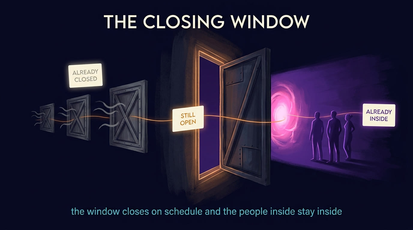
What is actually hard to copy
It is worth being precise about where the difficulty sits, because most of this is public. The mathematics is published. The papers are linked throughout this entry. The tools are documented, mostly free, and improving monthly. Anyone can read what is here.
What takes time is the convergence itself: holding the mathematics, an operational substrate to apply it through, and enough cross-domain exposure to notice that a decision problem in one field and a flow problem in another are the same object. Each of those makes the others more valuable, and none of them is fast. The scarce input is the years, and years are the one thing that cannot be bought at a discount.
Which makes the practical takeaway smaller and more useful than the framing suggests. You do not need the whole stack to get the benefit of the argument. Compute the ratio between how fast your environment moves and what it costs you to act, and let that set your posture instead of setting it in advance. Reach for the cheapest policy class that clears your bar. Put friction inside the calculation rather than subtracting it afterward. Keep the failures as structure rather than deleting them. Draw a hard line with creative work upstream of it and deterministic enforcement downstream. And keep the record of every run, because the record is what turns a pipeline into something that improves.
Each of those is independently useful, which is the property that made the metagraph migration tractable and makes this one tractable too. The unified picture is what explains why they belong together. Any single one of them pays for itself the week you adopt it.
The mathematics has been sitting there the whole time, indifferent to whether anyone picks it up. The window is the part that moves.